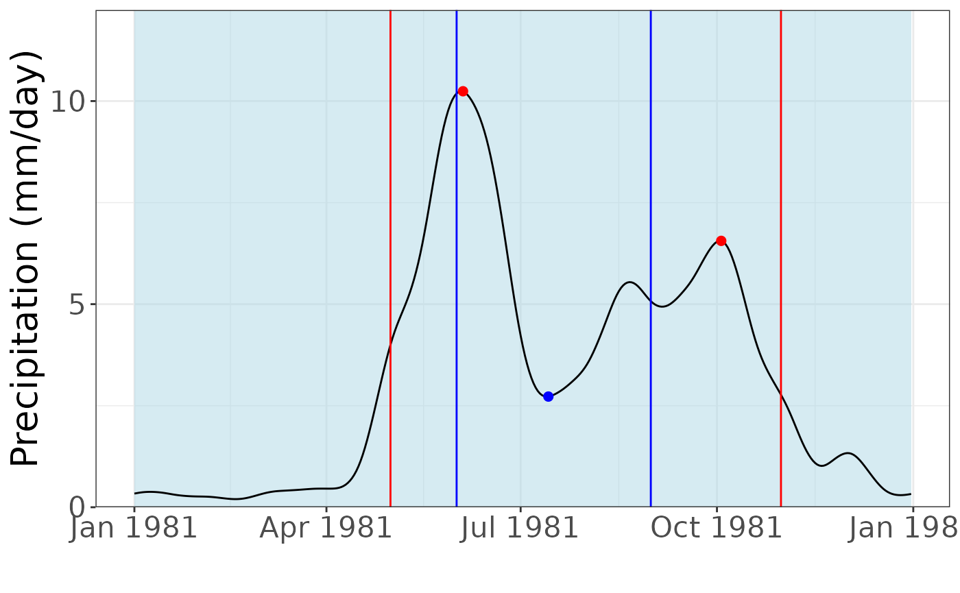
The msdrought package is designed to analyze one year of data at a time. For the AGU ’23 conference, a graphic was made that showcased the trends of the average rainfall across a set of years. Each day’s rainfall data across multiple years were averaged, then analyzed. For example, in a data set with precipitation data from 1981 to 1985, every day of the year (from January 1st to December 31st) had its rainfall data averaged (example: the precipitation values of 1-1-81, 1-1-82, 1-1-83, 1-1-84, and 1-1-85 were averaged), then put into a dummy xts to be analyzed. This vignette shows how that graphic was created.
The first step is to extract the relevant data from a SpatRaster.
library(tidyr)
#>
#> Attaching package: 'tidyr'
#> The following object is masked from 'package:terra':
#>
#>     extract
library(lubridate)
#>
#> Attaching package: 'lubridate'
#> The following objects are masked from 'package:terra':
#>
#>     intersect, union
#> The following objects are masked from 'package:base':
#>
#>     date, intersect, setdiff, union
library(stringr)
library(ggplot2)
library(xts)
#> Loading required package: zoo
#>
#> Attaching package: 'zoo'
#> The following object is masked from 'package:terra':
#>
#>     time<-
#> The following objects are masked from 'package:base':
#>
#>     as.Date, as.Date.numeric
data <- system.file("extdata", "prcp_cropped.tif", package = "msdrought") # This loads the data included in the package, but you would attach your own
infile <- terra::rast(data)

# Make a SpatRast for one point
lon <- -86.2621555581 # El Bramadero lon (from NicaAgua)
lat <- 13.3816217871 # El Bramadero lat (from NicaAgua)
lonLat <- data.frame(lon = lon, lat = lat)

# Set up precipitation data
location <- terra::vect(lonLat, crs = "+proj=longlat +datum=WGS84")
precip <- terra::extract(infile, location, method = "bilinear") %>%
  subset(select = -ID) %>%
  t()
precip[precip < 0] <- 0 # replace any negative (errant) values with zeroes
precip <- as.vector(precip)
Because we will be using the msdGraph function, a year value will need to be provided. We will create a dummy year that will be used for the sake of plotting. This can be any year, but it is easiest to just use the first year in the data set.
# Set up dates (time) data for ONE year (365 days)
allTimes <- terra::time(infile) %>%
  as.Date() %>%
  data.frame()
timeFrame <- as.Date(c(allTimes[1, 1]:allTimes[365, 1])) %>%
  data.frame()
# Make a Dataframe for each year
chunkLength <- 365
divYears <- (split(precip, ceiling(seq_along(precip) / chunkLength)))
divYearsFrame <- data.frame(divYears)

averagePrecip <- c()
for (i in 1:nrow(divYearsFrame)) {
  daySum <- sum(divYearsFrame[i, ])
  averagePrecip <- rbind(averagePrecip, daySum)
}
nyears <- round(length(precip) / 365)
averagePrecip <- averagePrecip / nyears # (average over number of years)
Now, an averaged xts object can be created. This will display the data set’s average rainfall over the dummy year.
# Assemble the Timeseries
timeseriesFrame <- cbind(timeFrame, averagePrecip)
colnames(timeseriesFrame) <- c("Date", "Precipitation")
x <- xts(timeseriesFrame$Precipitation, timeseriesFrame$Date) # This produces the "xts" screenshot
Now, perform the MSD calculations and plot the averaged graph!
# Perform MSD calculations with the new xts
keyDatesTS <- msdrought::msdDates(time(x))
filterTS <- msdrought::msdFilter(x, window = 31, quantity = 2)
duration <- msdrought::msdStats(filterTS, keyDatesTS, fcn = "duration")
#> Registered S3 method overwritten by 'quantmod':
#>   method            from
#>   as.zoo.data.frame zoo
intensity <- msdrought::msdStats(filterTS, keyDatesTS, fcn = "intensity")
firstMaxValue <- msdrought::msdStats(filterTS, keyDatesTS, fcn = "firstMaxValue")
secondMaxValue <- msdrought::msdStats(filterTS, keyDatesTS, fcn = "secondMaxValue")
min <- msdrought::msdStats(filterTS, keyDatesTS, fcn = "min")
allStats <- msdrought::msdMain(x)
graph1981 <- suppressWarnings(msdrought::msdGraph(x, 1981))
suppressWarnings(plot(graph1981))
# Note: suppressWarnings hides irrelevant messages that result from the msdGraph output